Eutropia
From ancient Greek, ευτροπία: docile, of good manners, versatile, variable.
The Point Spread Function (PSF) is a function that describes the pattern of light produced by a point-like source. In the context of NEXT, the PSF describes the fraction of charge (\(q_{rel}\)) detected by a SiPM as a function of the transverse distance (\(\Delta r = \sqrt{(\Delta x)^2 + (\Delta y)^2}\)) to the emission point. Even though in reality this is a continuous function, in practice we implement this function as a series of (\(\Delta r\), \(f\)) points, where \(f\) is the average fraction of detected light at a distance \(\Delta r\).
To obtain the PSF, we use \(^{83m}Kr\) events, due to their point-like nature. High energy electrons are not suitable for this task, due to their complex topology. \(^{83m}Kr\) events produce highly localized energy depositions (the closest we can achieve to a true point-like source) with fixed energy.
The PSF depends strongly on the z coordinate due to the effect of electron diffusion as they drift: it is narrower for short drift and wider for long drifts. Therefore, we do not produce a single PSF, but a collection of them, for different slices in z. The city has also the possibility of producing PSFs in different (x,y) sectors of the chamber to account for defects in the Tracking Plane.
PSFs are generated from Hits produced with a specific Penthesilea [1] configuration. For each z-slice and x,y-sector, the city produces the distribution of \(q_{rel}\) vs \(\Delta r\). This distribution is discretized in \(\Delta x\) and \(\Delta y\) bins and averaged over a large number of events.
The PSF is later used by Beersheba to reverse the effects of electron diffusion and light emission and obtain the original charge deposition.
Input
/Run/events: Table containing the event number and timestamps.
/Run/runInfo: Table containing the run number for each event.
/RECO/Events: Table containing the hits produced by Penthesilea.
Output
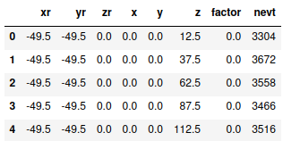
/PSF/PSFs: Table containing all the PSFs generated. Columns: xr, yr, zr, x, y, z, factor, nevt.
The columns xr, yr represent the center of each \(\Delta x\) and \(\Delta y\) bin, respectively. The column zr is always 0 and will be removed in the future. The columns x, y, and z indicate the center of the x-sector, y-sector and z-slice in which the PSF was generated. The columns factor and nevt are the PSF value and the number of events used to produce that number. This table might contain multiple PSFs (and it usually does), particularly for different z-slices.
Config
Besides the Common arguments to every city, Eutropia has the following arguments:
Parameter |
Type |
Description |
|---|---|---|
|
|
Ranges for the binning of \(\Delta x\) and \(\Delta y\). |
|
|
Bin edges for the z-slices. A set of PSFs (one for each x-y sector) will be produced in each bin. |
|
|
Bin edges for the x,y sectors. A PSF will be generated for each (x, y) sector and z-slice. |
|
|
Bin size for \(\Delta x\) and \(\Delta y\). |
Warning
A large ‘PSF size’ (defined by the xrange | yrange and
bin_size_xy) in conjunction with a large number of zbins
can cause excessive memory usage.
To avoid this issue, ensure that your xrange | yrange do not
exceed the PSF tails (~100mm for NEXT100), or use a smaller number
of zbins as a unique PSF is produced for each bin.
Workflow
Eutropia performs a number of data transformations in order to obtain the PSFs. These operations can be grouped in three main tasks, performed in the following order:
Prepare data slices
First, the events are grouped into x,y,z-slices according to the parameters zbins, xsectors and ysectors. Each of these sectors will have its own PSF [2]. These sectors can be identified in the output data by their central values (columns x, y and z of the output table). The procedure that follows is then applied to each of these datasets independently.
The hits coming from Penthesilea do not contain entries with null charge [3]. However, SiPMs with null charge should also be considered as part of the light response map. Thus, in this step, the missing hits are added to the dataset with zero charge. Next, the charge distribution is normalized to 1 for each event. Finally, the relative coordinates (\(\Delta x\) and \(\Delta y\)) are computed by subtracting the barycenter from each SiPM position.
Compute the PSFs
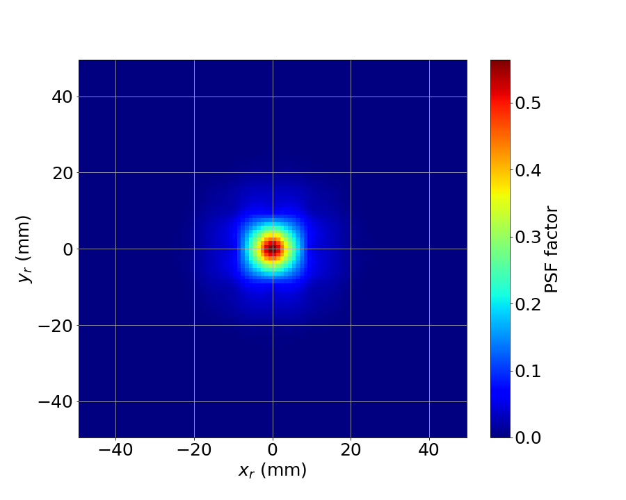
The charge distribution for all events is then histogrammed in \(\Delta x\) and \(\Delta y\). The binning of these histograms is determined by the parameters xrange, yrange, and bin_size_xy. The PSF factor in each bin is defined as the average normalized charge: \(\sum q_{rel} / n_{evt}\), where \(n_{evvt}\) is the number of events used to calculate the PSF factor. An example of such histogram is shown below.
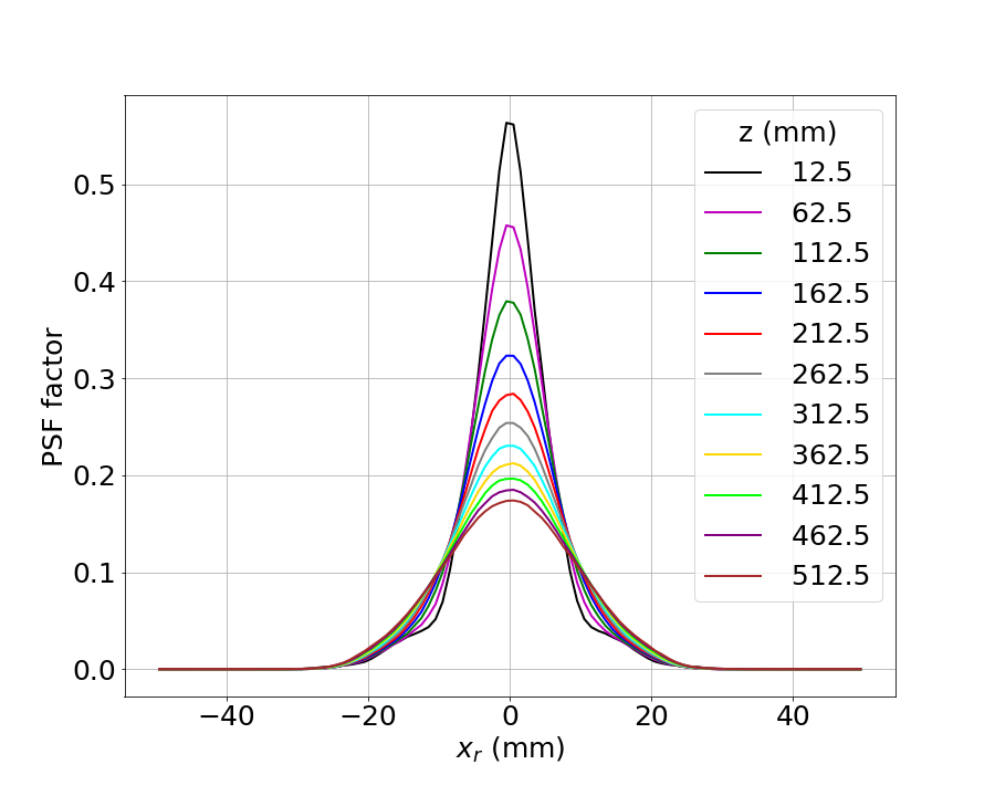
A 1d-slice of this histogram (for \(\Delta y = 0\)) is represented below for different z-slices, demonstrating why it is necessary to generate separate PSFs for various ranges of z.
Combine PSFs
In order to produce accurate PSF, a large number of events is necessary. At the same time, it is neither possible (in terms of memory) nor efficient to process a large number of events at once. The approach is thus to produce PSFs with the same parameters from fewer events and merge them afterwards. This option is available both within the city and externally as a separate tool. Because the city accepts many input files, it will run the PSF generation for each file independently and merge them later. The external tool follows the exact same methodology [4].
A PSF value is by construction an average of normalized charges. Therefore, an arbitrary number of PSF entries with values \(f_k\) produced with \(n_k\) events can be combined into a single entry with \(\sum_k n_k\) events and value